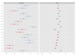
In the past week, colleagues of mine and me started using the lme4-package to compute multi level models. This inspired me doing two new functions for visualizing random effects (as retrieved by ranef()) and fixed effects (as retrieved by fixef()) of (generalized) linear mixed effect models.
The upcoming version of my sjPlot package will contain two new functions to plot fitted lmer and glmer models from the lme4 package: sjp.lmer and sjp.glmer (not that surprising function names). Since I’m new to mixed effects models, I would appreciate any suggestions on how to improve the functions, which results are important to report (plot) and so on. Furthermore, I’m not sure whether my approach of computing confident intervals for random effects is the best?
I have used following code to compute confident intervals for the estimates returned by the lme4::ranef() function (bases on this stackoverflow answer):
coev <- as.matrix(lme4::vcov.merMod(fit))
tmp <- as.data.frame(cbind(OR = exp(mydf.ef[,i]),
                     lower.CI = exp(mydf.ef[,i] - (1.96 * sqrt(diag(coev))[i])),
                     upper.CI = exp(mydf.ef[,i] + (1.96 * sqrt(diag(coev))[i]))))
The update to version 1.6 of sjPlot is still in development (feature-freeze, mostly fixes now), however, you can download the latest snapshot from GitHub (see also this post for further information). Now to some examples. First, an example model is fitted and the random effects (default) for each predictor are plotted as „forest plot“:
# fit model
library(lme4)
fit <- lmer(Reaction ~ Days + (Days | Subject), sleepstudy)
# simple plot
sjp.lmer(fit)
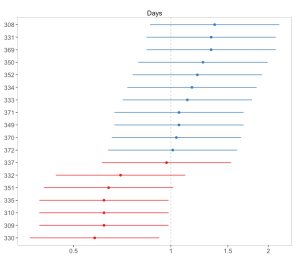
Sorting a predictor (i.e. estimates of a facet) is done by specifying the predictor’s name as sort parameter.
sjp.lmer(fit, sort = "Days")
Each facet plot can also be plotted as single plot, when facet.grid is set to FALSE. In this case, it is possible to sort the estimates for each plots. See following example from the sjp.glmer function:
library(lme4)
# create binary response
sleepstudy$Reaction.dicho <- sju.dicho(sleepstudy$Reaction,
                                       dichBy = "md")
# fit model
fit <- glmer(Reaction.dicho ~ Days + (Days | Subject),
             sleepstudy,
             family = binomial("logit"))
sjp.setTheme(theme = "forest")
sjp.glmer(fit,
          facet.grid = FALSE,
          sort = "sort.all")
Plotting the fixed effects is not much spectacular, because we only have one estimate beside intercept here.
sjp.glmer(fit,
          type = "fe",
          sort = TRUE)
To summarize, you can plot random and fixed effects in the way as shown above. Are there any other or better plot options for visualizing mixed effects models?
Any suggestions are welcome…
Disclaimer: all misspellings belong to Safari’s autocorrect feature!


There is a way to calculate Standard Errors for the random effects in the arm package
Thanks for the hint! I included the se.ranef function from the arm-package.
function invlogit is useful and it is in arm package too. I’m thinking in a way to plot probabilities instead log odds.
I guess you mean something like what is implemented in the
sjp.glmfunction? See the sjp.glm examples, last paragraph Probabilities of continuous variables. Based on this stack exchange discussion, I have implemented a function to plot probabilities of continuous predictors of logistic regressions.invlogitandsjPlot:::odds.to.probyield exactly the same values – invlogit uses 1/(1 + exp(-x)), while I use exp(x)/(1+exp(x)). I may implement this for sjp.glmer as well, however, I need to get more familiar with glmerMod-objects to know how to extract continuous predictors from those objects.Does it work when there are two (or mode) random-effects terms??? y ~ 1 + (1 | municipality) + (1 | healthfacility), …, and what about the visualization when levels are nested vs non-nested?
I can’t say that for sure by now, because I haven’t worked much with mixed effects models yet, so I can’t predict how the ranef and fixef function work. But I’ll keep updating the functions to add different use cases…
mo2 <- glmer(ancone ~ agmo+agfcb+time*treatment + (1 | vdc), data = mch,family = binomial(link = "logit"), nAGQ = 25)
summary(mo2)
sjp.glmer(mo2, type="fe")
i go the error for the fixed effect plot but i got random effect plot
Error in `$<-.data.frame`(`*tmp*`, "p", value = c("7.59 ***", "0.92 ***", :
replacement has 6 rows, data has 7
In addition: Warning message:
In cbind(OR = lme4::fixef(fit), lme4::confint.merMod(fit, method = "Wald")) :
number of rows of result is not a multiple of vector length (arg 1)
You have to update the packages, I assume it’s due to a change in the lme4-package.
Dear Daniel
Thank you very much, it works
Dear Daniel.
This visualization was easy to understand for me.
I want to try „secret weapon“ by Gelman.
However, I could not.
Code;
theDays <- unique(sleepstudy$Days)
results <- vector(mode = "list", length = length(theDays))
names(results) <- theDays
for(i in theDays){
results[[as.character(i)]] <- lmer(Reaction ~ Days + (Days | Subject),
data = sleepstudy, subset = Days ==i)
}
Error;
number of levels of each grouping factor must be < number of observations
What's wrong?
Best regards,
Masa
That is an issue with lme4 resp. your model specification. Your random slope has to be continuous.
Dear Daniel
Is there any command to get the ICC (Intraclass correlation coefficient) for multilevel model of lme4 package.
Thanks
Yes, see
icc()in my sjstats package.