Quickly create Codeplans of your (labelled) Data #rstats

The view_df() function from the sjPlot-package creates nice „codeplans“ from your data sets, and also supports labelled data and tagged NA-values. This gives you a comprehensive, yet clear overview of your data set.

To demonstrate this function, we use a (labelled) data set from the European Social Survey. view_df() produces a HTML-file, that is – when you use RStudio – displayed in the viewer pane, or it can be opened in your webbrowser.

ggeffects 0.8.0 now on CRAN: marginal effects for regression models #rstats

I’m happy to announce that version 0.8.0 of my ggeffects-package is on CRAN now. The update has fixed some bugs from the previous version and comes along with many new features or improvements. One major part that was addressed in the latest version are fixed and improvements for mixed models, especially zero-inflated mixed models (fitted with the glmmTMB-package).

In this post, I want to demonstrate the different options to calculate and visualize marginal effects from mixed models.

Marginal Effects for (mixed effects) regression models #rstats

ggeffects (CRAN, website) is a package that computes marginal effects at the mean (MEMs) or representative values (MERs) for many different models, including mixed effects or Bayesian models. One of the advantages of the package is its easy-to-use interface: No matter if you fit a simple or complex model, with interactions or splines, the function call is always the same. This also holds true for the returned output, which is always a data frame with the same, consistent column names.

The past package-update introduced some new features I wanted to describe here: a revised print()-method as well as a new opportunity to plot marginal effects at different levels of random effects in mixed models…

R functions for Bayesian Model Statistics and Summaries #rstats #stan #brms

A new update of my sjstats-package just arrived at CRAN. This blog post demontrates those functions of the sjstats-package that deal especially with Bayesian models. The update contains some new and some revised functions to compute summary statistics of Bayesian models, which are now described in more detail.

• hdi()
• rope()
• mcse()
• n_eff()
• tidy_stan()
• equi_test()
• mediation()
• icc()
• r2()

Before we start, we fit some models, including a mediation-object from the mediation-package, which we use for comparison with brms. The functions work with brmsfit, stanreg and stanfit-objects.

Anova-Freak and Bayesian Hipster #rstats

I’m pleased to announce an update of my sjstats-package. New features are specifically implemented for the Anova and Bayesian statistic and summary functions. Here’s a short overview of what’s new…

Data transformation in #tidyverse style: package sjmisc updated #rstats

I’m pleased to announce an update for the sjmisc-package, which was just released on CRAN. Here I want to point out two important changes in the package.

New default option for recoding and transformation functions

First, a small change in the code with major impact on the workflow, as it affects argument defaults and is likely to break your existing code – if you’re using sjmisc: The append-argument in recode and transformation functions like rec(), dicho(), split_var(), group_var(), center(), std(), recode_to(), row_sums(), row_count(), col_count() and row_means() now defaults to TRUE.

The reason behind this change is that, in my experience and workflow, when transforming or recoding variables, I typically want to add these new variables to an existing data frame by default. Especially in a pipe-workflow, when I start my scripts with importing and basic tidying of my data, I almost always want to append the recoded variables to my existing data, e.g.:

# Example with following steps:
# 1. loading labelled data set
# 2. dropping unused labels
# 3. converting numeric into categorical, using labels as levels
# 4. center some variables
# 5. recode some other variables
data %>%
  drop_labels() %>%
  as_label(var1:var5) %>%
  center(var7, var9) %>%
  rec(var11, rec = "2=0;1=1;else=copy")

Bayesian Regression Modelling in R: Choosing informative priors in rstanarm #rstats

Yesterday, at the last meeting of the Hamburg R User Group in this year, I had the pleasure to give a talk about Bayesian modelling and choosing (informative) priors in the rstanarm-package.

You can download the slides of my talk here.

Thanks to the Stan team and Tristan for proof reading my slides prior (<- hoho) to the talk. Disclaimer: Still, I'm fully responsible for the content of the slides, and I'm to blame for any false statements or errors in the code…

„One function to rule them all“ – visualization of regression models in #rstats w/ #sjPlot

I’m pleased to announce the latest update from my sjPlot-package on CRAN. Beside some bug fixes and minor new features, the major update is a new function, plot_model(), which is both an enhancement and replacement of sjp.lm(), sjp.glm(), sjp.lmer(), sjp.glmer() and sjp.int(). The latter functions will become deprecated in the next updates and removed somewhen in the future.

plot_model() is a „generic“ plot function that accepts many model-objects, like lm, glm, lme, lmerMod etc. It offers various plotting types, like estimates/coefficient plots (aka forest or dot-whisker plots), marginal effect plots and plotting interaction terms, and sort of diagnostic plots.

In this blog post, I want to describe how to plot estimates as forest plots.

My set of packages for (daily) data analysis #rstats

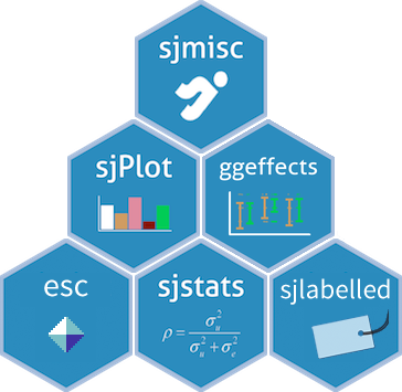
I started writing my first package as collection of various functions that I needed for (almost) daily work. Meanwhile, packages were growing and bit by bit I sourced out functions to put them into new packages. Although this means more work for CRAN members when they have more packages to manage on their network, from a user-perspective it is much better if packages have a clear focus and a well defined set of functions. That’s why I now released a new package on CRAN, sjlabelled, which contains all functions that deal with labelled data. These functions use to live in the sjmisc-package, where they now are deprecated and will be removed in a future update.

My aim is not only to provide packages with a clear focus, but also with a consistent design and philosophy, making it easier and more intuitive to use (see also here) – I prefer to follow the so called „tidyverse“-approach here. It is still work in progress, but so far I think I’m on a good way…

So, what are the packages I use for (almost) daily work?

• sjlabelled – reading, writing and working with labelled data (especially since I collaborate a lot with people who use Stata or SPSS)
• sjmisc – data and variable transformation utilities (the complement to dplyr and tidyr, when it comes down from data frames to variables within the data wrangling process)
• sjstats – out-of-the-box statistics that is not already provided by base R or packages
• sjPlot – to quickly generate tables and plot
• ggeffects – to visualize regression models

The next step is creating cheat sheets for my packages. I think if you can map the scope and idea of your package (functions) on a cheat sheet, its focus is probably well defined.

Btw, if you also use some of the above packages more or less regularly, you can install the „strengejacke“-package to load them all in one step. This package is not on CRAN, because its only purpose is to load other packages.

Disclaimer: Of course I use other packages everyday as well – this posting is just focussing on my packages that I created because I frequently needed these kind of functions.

ggeffects: Create Tidy Data Frames of Marginal Effects for ‚ggplot‘ from Model Outputs #rstats

Aim of the ggeffects-package

The aim of the ggeffects-package is similar to the broom-package: transforming “untidy” input into a tidy data frame, especially for further use with ggplot. However, ggeffects does not return model-summaries; rather, this package computes marginal effects at the mean or average marginal effects from statistical models and returns the result as tidy data frame (as tibbles, to be more precisely).

Since the focus lies on plotting the data (the marginal effects), at least one model term needs to be specified for which the effects are computed. It is also possible to compute marginal effects for model terms, grouped by the levels of another model’s predictor. The package also allows plotting marginal effects for two- or three-way-interactions, or for specific values of a model term only. Examples are shown below.